Magma Sanctum

複素関数論による連続体力学

任意形状鉄心の空隙磁束分布の解析的計算法

この記事は、書きかけの記事です。(電動機の一般論について勉強中)


この記事の目的は、”とにかく解析的に”空隙境界に生じるマクスウェルの応力分布を求めたい、ということです。


電動機トルクは鉄心に発生するトルクと巻線に発生するトルクに大きく分けられますが、本記事では前者について扱っています。

複素磁位および等角写像法を用いて空隙磁束分布を解析的計算する方法は既に示されていますが、Schwarz-Christoffel変換を用いた多角形の写像に関するものが大半で任意形状鉄心を対象としたものは見当たりません。*1


そこで、本方法では空隙境界に生じる磁位差を入力してマクスウェルの応力を出力することを目的に、前回導出した任意の境界条件に対する複素関数論を応用します。

magma-sanctum.hatenablog.com


・複素磁位の導出


f:id:Magma_Sanctum:20220224041413j:plain


 z 平面(単位円)で境界条件を決定し、 \zeta 平面(物理面)に等角写像する方法

最終的に空隙部の局所磁束密度を

 \left( \dfrac {d f}{d \zeta} \right) _R = \dfrac {d f}{d \theta} \cdot \dfrac {d \theta}{d \zeta} = \left. \dfrac {d f}{d \theta} \right/ \left( \dfrac {d \xi}{d \theta} + i \dfrac {d \eta}{d \theta} \right)

とすることで、磁束密度の項を空隙形状(鉄心形状)の項から分離して導出する

※空隙形状の関数はフーリエ級数展開により導出(前回記事を参照)


複素磁位 f  z=0周りで( z \rightarrow \infty で発散しないように)展開すると

 f = \phi + i \psi = s \log z + \left( B_x - i B_y \right) z + \displaystyle \sum_{1}^{\infty} \left( P_n + i Q_n \right) z^{- n}

 \phi = Re ( s ) \log r - Im ( s ) \theta + r \left( B_x \cos \theta + B_y \sin \theta \right) + \displaystyle \sum_{0}^{\infty} r^{- n} \left( P_n \cos n \theta + Q_n \sin n \theta \right)

周方向磁束密度は

 B_\theta = \dfrac {1}{r} \dfrac {\partial \phi}{\partial \theta} = - \dfrac {Im ( s )}{r} - B_x \sin \theta + B_y \cos \theta + \displaystyle \sum_{0}^{\infty} n r^{- n - 1} \left( - P_n \sin n \theta + Q_n \cos n \theta \right)


ここで、単位円上( r = R ( = 1 / 2 ) )の周方向磁束密度分布に境界条件として b_\theta ( \theta ) を与えフーリエ級数展開することで係数比較をする

 \dfrac {Im ( s )}{R} = - \dfrac {1}{2 \pi} \displaystyle \int_{0}^{2 \pi} b_\theta \, d \theta

 B_x + \dfrac {P_1}{R^2} = - \dfrac {1}{\pi} \displaystyle \int_{0}^{2 \pi} b_\theta \sin \theta \, d \theta ,  B_y + \dfrac {Q_1}{R^2} = \dfrac {1}{\pi} \displaystyle \int_{0}^{2 \pi} b_\theta \cos \theta \, d \theta

 n R^{-n-1} P_n = - \dfrac {1}{\pi} \displaystyle \int_{0}^{2 \pi} b_\theta \sin ( n \theta ) \, d \theta ,  n R^{-n-1} Q_n = \dfrac {1}{\pi} \displaystyle \int_{0}^{2 \pi} b_\theta \cos ( n \theta ) \, d \theta


複素速度ポテンシャルに係数を戻して

 f = \left( Re ( s ) + i Im ( s ) \right) \left( \log R + i \theta \right) + \left( r - \dfrac {R^2}{r} \right) \left( B_x \cos \theta +B_y \sin \theta \right) + i \left( r + \dfrac {R^2}{r} \right) \left( - B_y \cos \theta + B_x \sin \theta \right) \\ + \dfrac {R}{\pi} \displaystyle \sum_{1}^{\infty} \dfrac {1}{n} \left( \dfrac {R}{r} \right)^n \left( - \displaystyle \int_{0}^{2 \pi} b_\theta \sin ( n \theta ) \, d \theta + i \displaystyle \int_{0}^{2 \pi} b_\theta \cos ( n \theta ) \, d \theta \right) \left( \cos n \theta - i \sin n \theta \right)


以降 r = R ( = 1 / 2 ) として

 \dfrac {d f}{d \theta} = \left( - Im ( s ) + i Re ( s ) \right) + 2 i R \left( B_x \cos \theta + B_y \sin \theta \right) \\ + \dfrac {R}{\pi} \displaystyle \sum_{1}^{\infty} \left( \displaystyle \int_{0}^{2 \pi} b_\theta \sin ( n \theta ) \, d \theta - i \displaystyle \int_{0}^{2 \pi} b_\theta \cos ( n \theta ) \, d \theta \right) \left( \sin n \theta + i \cos n \theta \right)


磁束密度場を実部(周方向磁束密度であり磁位差に相当)と虚部(半径方向磁束密度)に分ける

 \dfrac {d \phi}{d \theta} = \dfrac {R}{2 \pi} \displaystyle \int_{0}^{2 \pi} b_\theta \, d \theta + \dfrac {R}{\pi} \displaystyle \sum_{1}^{\infty} \left \{ \left( \displaystyle \int_{0}^{2 \pi} b_\theta \sin ( n \theta ) \, d \theta \right) \sin n \theta + \left( \displaystyle \int_{0}^{2 \pi} b_\theta \cos ( n \theta ) \, d \theta \right) \cos n \theta \right \} = R b_\theta ( \theta )

 \dfrac {d \psi}{d \theta} = Re ( s ) + 2 R \left( B_x \cos \theta + B_y \sin \theta \right) - \dfrac {R}{\pi} \displaystyle \sum_{1}^{\infty} \left \{ \left( - \displaystyle \int_{0}^{2 \pi} b_\theta \sin ( n \theta ) \, d \theta \right) \cos n \theta + \left( \displaystyle \int_{0}^{2 \pi} b_\theta \cos ( n \theta ) \, d \theta \right) \sin n \theta \right \} \\ = Re ( s ) + 2 R \left( B_x \cos \theta + B_y \sin \theta \right) - R {b_\theta}^*

(ここで {b_\theta}^* ( \theta ) は”共役フーリエ級数”)


よって、半径方向磁束密度は以下のように求められた

 b_r ( \theta ) = \dfrac {Re ( s )}{R} + 2 \left( B_x \cos \theta + B_y \sin \theta \right) + \dfrac {1}{2 \pi} \displaystyle \int_{0}^{2 \pi} \left( b_\theta ( \varphi ) -b_\theta ( \theta ) \right) \cot \dfrac {\varphi - \theta}{2} \, d \theta


ここで、周方向磁束密度 b_\theta ( \theta ) は磁位差に由来し、巻線電流から決定する*2

また、マクスウェルの応力は鉄心の透磁率が無限大であると仮定して次のように求められる

 p = \left. \dfrac {1}{2 \mu_0} {b_r}^2 ( \theta ) \right/ g ( \theta )

 \mu_0 は空隙の透磁率


空隙を介して回転子と固定子に働くトルクが打ち消し合うことを考えると、マクスウェルの応力の空隙輪郭に沿った積は零になると考えられます。


(閉スロットおよび永久磁石の場合を考察中のため、今後追記する予定です)


剥離を伴った任意翼型まわりの流れの解析的計算法

この記事の目的は、”とにかく解析的に”剥離を伴う翼の圧力分布を求めたい、ということです。


剥離を伴う流れを比較的解析的に計算する方法としては、境界要素法、自由流線理論、離散渦法、などが挙げられますが、結局いずれにせよ計算段階でパネル分割することになることがほとんどです。(最後まで解析的な導出法は見たことがない)


試行錯誤を繰り返すうちに、解析的に解くための条件は、(1)ポテンシャル流れであること、(2)単独翼であること、(3)境界条件が明確であること、と分かってきました。


そこで、本方法では剥離領域の排除効果を吹き出し流れによって近似することで導出します。(”wake source method”)*1


・さっそく導出してみる


最終的に翼面上の局所流速を

 \left( \dfrac {d f}{d \zeta} \right) _R = \dfrac {d f}{d \theta} \cdot \dfrac {d \theta}{d \zeta} = \left. \dfrac {d f}{d \theta} \right/ \left( \dfrac {d \xi}{d \theta} + i \dfrac {d \eta}{d \theta} \right)

とすることで、流れの項を翼型の項から分離して導出する


翼型の関数は守屋富次郎先生の「空気力学序論」を参考にして翼型をフーリエ級数展開することで次のように求められる。

 g ( \theta ) = \dfrac {d \xi}{d \theta}^2 + \dfrac {d \eta}{d \theta}^2 = \dfrac {1}{4} \sin ^{2} \theta + \left \{ - \displaystyle \sum_{1}^{\infty} n A_n \sin n \theta + \displaystyle \sum_{1}^{\infty} n B_n cos n \theta \right \}^2


複素速度ポテンシャルを z=0周りで( z \rightarrow \infty で発散しないように)展開すると

 f = \phi + i \psi = s \log z + \left( u - i v \right) z + \displaystyle \sum_{1}^{\infty} \left( P_n + i Q_n \right) z^{- n}

 \phi = Re ( s ) \log r - Im ( s ) \theta + r \left( u \cos \theta + v \sin \theta \right) + \displaystyle \sum_{0}^{\infty} r^{- n} \left( P_n \cos n \theta + Q_n \sin n \theta \right)

半径方向速度は

 \dfrac {\partial \phi}{\partial r} = \dfrac {Re ( s )}{r} + u \cos \theta + v \sin \theta - \displaystyle \sum_{0}^{\infty} n r^{- n - 1} \left( P_n \cos n \theta +Q_n \sin n \theta \right)


ここで、単位円上( r = R ( = 1 / 2 ) )の垂直速度分布に境界条件として吹き出し分布 v_r ( \theta ) を与えフーリエ級数展開することで係数比較をする

 \dfrac {Re ( s )}{R} =\dfrac {1}{2 \pi} \displaystyle \int_{0}^{2 \pi} v_r \, d \theta

 u - \dfrac {P_1}{R^2} = \dfrac {1}{\pi} \displaystyle \int_{0}^{2 \pi} v_r \cos \theta \, d \theta ,  v - \dfrac {Q_1}{R^2} = \dfrac {1}{\pi} \displaystyle \int_{0}^{2 \pi} v_r \sin \theta \, d \theta

 - n R^{-n-1} P_n = \dfrac {1}{\pi} \displaystyle \int_{0}^{2 \pi} v_r \cos ( n \theta ) \, d \theta ,  - n R^{-n-1} Q_n = \dfrac {1}{\pi} \displaystyle \int_{0}^{2 \pi} v_r \sin ( n \theta ) \, d \theta


複素速度ポテンシャルに係数を戻して

 f = \left( Re ( s ) + i Im ( s ) \right) \left( \log R + i \theta \right) + 2 R \left( u \cos \theta + v \sin \theta \right) \\ - \dfrac {R}{\pi} \displaystyle \sum_{1}^{\infty} \dfrac {1}{n} \left( \displaystyle \int_{0}^{2 \pi} v_r \cos ( n \theta ) \, d \theta + i \displaystyle \int_{0}^{2 \pi} v_r \sin ( n \theta ) \, d \theta \right) \left( \sin n \theta + i \cos n \theta \right)

 \dfrac {d f}{d \theta} = \left( - Im ( s ) + i Re ( s ) \right) - 2 R \left( \log R + i \theta \right) \\ + \dfrac {R}{\pi} \displaystyle \sum_{1}^{\infty} \left( \displaystyle \int_{0}^{2 \pi} v_r \cos ( n \theta ) \, d \theta + i \displaystyle \int_{0}^{2 \pi} v_r \sin ( n \theta ) \, d \theta \right) \left( \sin n \theta + i \cos n \theta \right)


速度場を実部(接線速度分布)と虚部(垂直速度分布)に分ける

 Re \left( \dfrac {d f}{d \theta} \right) = - Im ( s ) - 2 R \left( u \sin \theta - v \cos \theta \right) \\ + \dfrac {R}{\pi} \displaystyle \sum_{1}^{\infty} \left \{ \left( - \displaystyle \int_{0}^{2 \pi} v_r \sin ( n \theta ) \, d \theta \right) \cos n \theta + \left( \displaystyle \int_{0}^{2 \pi} v_r \cos ( n \theta ) \, d \theta \right) \sin n \theta \right \} \\ = - Im ( s ) - 2 R \left( u \sin \theta - v \cos \theta \right) + R {v_r}^* ( \theta )

 Im \left( \dfrac {d f}{d \theta} \right) = Re ( s ) + \dfrac {R}{\pi} \displaystyle \sum_{1}^{\infty} \left \{ \left( - \displaystyle \int_{0}^{2 \pi} v_r \cos ( n \theta ) \, d \theta \right) \cos n \theta + \left( \displaystyle \int_{0}^{2 \pi} v_r \sin ( n \theta ) \, d \theta \right) \sin n \theta \right \} \\ = Re ( s ) + R v_r ( \theta ) - \dfrac {R}{2 \pi} \displaystyle \int_{0}^{2 \pi} v_r ( \theta ) \, d \theta = R v_r ( \theta )


ここで {v_r}^* ( \theta ) フーリエ級数余弦と正弦を入れ替えた関数となっているが、これは”共役フーリエ級数”であり今井功先生の「等角写像とその応用」によれば次のように変換できる

 Re \left( \dfrac {d f}{d \theta} \right) = - Im ( s ) - 2 R \left( u \sin \theta - v \cos \theta \right) - \dfrac {R}{2 \pi} \displaystyle \int_{0}^{2 \pi} \left( v_r ( \varphi ) - v_r ( \theta ) \right) \cot \dfrac {\varphi - \theta}{2} \, d \varphi


よって、求めるべき局所流速分布は次のようになる(意外とシンプルな式にまとまった)

 q^2 = \left. \left [ Re \left( \dfrac {d f}{d \theta} \right)^2 + Im \left( \dfrac {d f}{d \theta} \right)^2 \right ] \right/ g ( \theta ) \\ = \left. \left [ \left \{ Im ( s ) + 2 R \left( u \sin \theta - v \cos \theta \right) + \dfrac {R}{2 \pi} \displaystyle \int_{0}^{2 \pi} \left( v_r ( \varphi ) - v_r ( \theta ) \right) \cot \dfrac {\varphi - \theta}{2} \, d \varphi \right \}^2 + \left \{ R v_r ( \theta ) \right \}^2 \right ] \right/ g ( \theta )

 Im ( s ) は循環成分であり、クッタの条件により決まる


剥離点 \alpha と再付着点 \beta を持つ剥離泡を近似するには、流れ関数が一定の時( \psi = const. )流線が一致するので

 \Delta \psi = \displaystyle \int_{\alpha}^{\beta} Im \left( \dfrac {d f}{d \theta} \right) \, d \theta = R \displaystyle \int_{\alpha}^{\beta} v_r ( \theta ) \, d \theta = 0

を満たす吹き出し分布 v_r 境界条件として与えればよい


・計算例 


Excel表計算機能で圧力分布を導出してみました。


以下のグラフは入力した吹き出し分布と出力した共役フーリエ級数の比較です。

f:id:Magma_Sanctum:20210714140624p:plain

剥離泡の流速への影響が剥離領域に限られていることがわかります。「short bubble は翼型全体にわたる potential flow としての圧力分布にはあまり影響を与えない」*2という経験則と良い一致を示しています。

また、 圧力分布は次のようになりました。

f:id:Magma_Sanctum:20210714140958p:plain

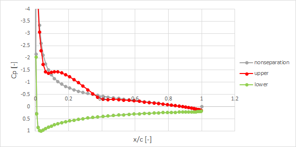
注意しなくてはいけないのが、いかにも剥離泡の特性である圧力一定領域と圧力回復を示しているように見えますが、あくまでも排除効果を利用した計算であり、この剥離領域においては特に意味のあるものではないです。

吹き出し分布と逆流域の関係は考察中です)